Abstract
This study reveals the thermal behavior of an unsteady nanofluid streaming between two parallel plates by using artificial neural network (ANN). Initially, a similarity solution is employed to simplify the partial differential equations (PDSs) and convert them into a system of coupled nonlinear ordinary differential equations (ODEs). Subsequently, a numerical analysis is undertaken to verify the predicted results applying forth order Runge Kutta method. ANN is utilized to provide a nonlinear map between the considered input parameters such as solid volume fraction (Φ), Eckert number (Ec) and a moving parameter which represents the movement of the parallel plates (S), and output parameters like Nusselt number (Nu). Considering the accuracy of the current results, it is concluded that ANN method can be a potential reliable approach for function approximation. Results indicate that an optimal network with 16 neurons exists in hidden layer for which the value of RMSE for testing data is found to be 0.001364.
License
This is an open access article distributed under the Creative Commons Attribution License which permits unrestricted use, distribution, and reproduction in any medium, provided the original work is properly cited.
Article Type: Research Article
EUR J SUSTAIN DEV RES, Volume 3, Issue 1, 2019, Article No: em0069
https://doi.org/10.20897/ejosdr/3935
Publication date: 06 Feb 2019
Online publication date: 31 Oct 2018
Article Views: 6112
Article Downloads: 3001
Open Access HTML Content References How to cite this articleHTML Content
INTRODUCTION
Accurate anticipation of the behavior of fluid flows and heat transfer can remove harmful effects such as mechanical noises and vibrations from industrial systems (Jianu and Rosen, 2017; Shahriari et al., 2018). Fluid heating and cooling are important inevitable processes extensively occurring in many industries such as power, manufacturing and transportation. Due to their low heat transfer properties, common heat transfer fluids such as water, ethylene glycol, and engine oil suffer from relatively inappropriate heat transfer properties. On the other hand, in some cases, thermal conductivity of metals is up to three times higher than the aforementioned fluids. Therefore, mixing of stable and desirable substances can be a potential technique for reaching high thermal conductivities.
So far, it has been proven in numerous research studies that nanofluids can be superior when they are utilized as a heat transfer agent over conventional fluids (Kumar et al., 2014; Kim, 2014; Kumar et al., 2015; Muthtamilselvan et al., 2014).
Sheikholeslami et al. (2012) investigated the heat transfer characteristics of nanofluids flow between two horizontal plates in a rotating system. Their results showed that for suction and injection, the heat transfer rate at the surface rises with enhancing the nanoparticle volume fraction, Reynolds number, and injection/suction parameter, and declines with power of rotation parameter. Azimi et al. (2014) examined the effects of solid volume fraction of a nanoparticle, moving parameter and Eckert number on heat transfer behavior of nanofluid flow between two moving parallel plates. In another study conducted by Azimi et al. (2015), MHD Jeffery Hamel flow problem with a nanoparticle was presented for several different values of Hartman number.
The major goal of enhanced heat transfer is to encourage high heat fluxes (Eiamsa-ard and Changcharoen, 2015). In a report presented by Lihong and Hangmingthe (Lihong and Hangming, 2015), for enhancing heat transfer from walls to the interior and improving the isothermal characteristics of the isothermal chamber, distribution of thin copper wire in an isothermal chamber was described using topological methods.
Moslehi and Saghafian (2015) numerically examined mixed convection heat transfer of a steady laminar flow of a Newtonian conductive fluid in an open-ended vertical parallel microchannel considering a uniform magnetic field.
Azimi and Riazi (2015) employed an analytical method, namely Galerkin Optimal Homotopy Asymptotic Method (GOHAM), to discover the approximate solution of an unsteady MHD squeezing flow between two parallel disks. They presented that average Nusselt number is an increasing function of nanoparticle volume fraction as well as Rayleigh number, while it is a decreasing function of Hartmann number. Thermal analysis of an unsteady nanofluid flow between two moving parallel plates was conducted by Azimi and Mozaffari utilizing intelligent black-box identifier (Azimi and Mozaffari, 2015). Free convection boundary layer in a steady magneto-hydrodynamic flow through a vertical semi-infinite flat plate embedded in water and filled with a nanofluid was theoretically investigated by Hamad et al. (2011). They found that Cu and Ag nanoparticles possessed the highest cooling performance in the considered problem. Sheikholeslami et al. (2012) performed a numerical analysis to study the natural convection heat transfer of Cu-water nanofluid in a circular enclosure surrounding a hot sinusoidal circular cylinder in presence of horizontal magnetic field using a Finite Element Method. The effect of viscous dissipation on temperature distribution of a two-dimensional unsteady nanofluid flow between two moving parallel plates was analytically studied by Shahriari et al. (2018). Sheikholeslami et al. (2013) determined the behavior of an unsteady nanofluid flow between two parallel plates applying Adomain Decomposition Method (ADM) (Sheikholeslami et al., 2013). According to their results, for the case in which both of the plates are moveable, Nusselt number decreases with an increment in squeeze number and grows with increasing the nanoparticle volume fraction and Eckert number. Sheikholeslami and Ganji (2013) employed Homotopy Perturbation Method to peruse the thermal behavior of a nanofluid squeezing flow (Sheikholeslami and Ganji, 2013). Based on their results, Nusselt number directly depended on the nanoparticle volume fraction, squeeze and Eckert numbers when plates are separated and inversely depended on squeeze number when the plates are squeezed. Rahimi-Gorji et al. (2016) employed Galerkin method (GM) to solve nonlinear differential equations for an unsteady squeezing nanofluid flow taking into account variable magnetic field (2016). With regard to their results, with an enhancement in nanofluid volume fraction Nusselt number increased while skin friction coefficient declined. In addition, an increment in the value of nanofluid volume fraction led to increments in the values of flow velocity and temperature. The main aim of the current study is to discuss the heat transfer solutions of a two-dimensional nanofluid sueezing flow between two moving parallel plates.
PROBLEM DESCRIPTION
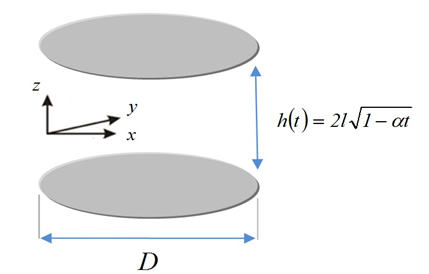
In this section, as can be seen in Figure 1, we describe the unsteady 2D squeezing flow and heat transfer of a nanofluid between two infinite plates.
|
Table 1. Thermophysical properties of water and the nanoparticle
|
The viscous dissipation impact occurring in high Eckert numbers and heat generation caused by shear stress in the flow are retained. Eckert number expresses the relationship between kinetic energy and enthalpy of flows. Table 1 lists the properties of the considered fluid (water) and a nanoparticle. As can be observed in Figure 1, the two plates are located at\(z = \pm l\left( 1 - \alpha t \right)^{\frac{1}{2}} = \pm h\left( t \right)\). The unsteady equations of mass conservation and momentum can be expressed as follows (Shahriari et al., 2018):
| \[\frac{\partial u}{\partial x} + \frac{\partial v}{\partial y} = 0\] | (1) |
| \[\rho_{\text{nf}}\left( \frac{\partial u}{\partial t} + u\frac{\partial u}{\partial x} + u\frac{\partial u}{\partial y} \right) = - \frac{\partial p}{\partial x} + \mu_{\text{nf}}\left( \frac{\partial^{2}u}{\partial x^{2}} + \frac{\partial^{2}u}{\partial y^{2}} \right)\] | (2) |
| \[\rho_{\text{nf}}\left( \frac{\partial v}{\partial t} + u\frac{\partial v}{\partial x} + v\frac{\partial v}{\partial y} \right) = - \frac{\partial p}{\partial y} + \mu_{\text{nf}}\left( \frac{\partial^{2}v}{\partial x^{2}} + \frac{\partial^{2}v}{\partial y^{2}} \right)\] | (3) |
| \[\frac{\partial T}{\partial t} + u\frac{\partial T}{\partial x} + v\frac{\partial T}{\partial y} = \frac{k_{\text{nf}}}{\left( \rho C_{p} \right)_{\text{nf}}}\left( \frac{\partial^{2}T}{\partial x^{2}} + \frac{\partial^{2}T}{\partial y^{2}} \right) + \frac{\mu_{\text{nf}}}{\left( \rho C_{p} \right)_{\text{nf}}}\left\lbrack 4\left( \frac{\partial u}{\partial x} \right)^{2} + \left( \frac{\partial u}{\partial x} + \frac{\partial u}{\partial y} \right)^{2} \right\rbrack\] | (4) |
where \(u\) and \(v\) are velocities in \(x\) and \(y\) directions, respectively. Effective density (\(\rho_{\text{nf}}\)), effective dynamic viscosity (\(\mu_{\text{nf}}\)), effective heat capacity \(\left( \rho C_{p} \right)_{\text{nf}}\) and effective thermal conductivity \(k_{\text{nf}}\) of the nanofluid can be defined as follows (Hamad et al., 2011):
| \[\left\{ \begin{matrix} \rho_{\text{nf}} = \rho_{f}\left( 1 - \phi \right) + \rho_{s}\phi_{s} \\ \left( \rho C_{p} \right)_{\text{nf}} = \left( \rho C_{p} \right)_{f}\left( 1 - \phi \right) + \left( \rho C_{p} \right)_{s} \\ \mu_{\text{nf}} = \frac{\mu_{f}}{\left( 1 - \phi \right)^{2.5}} \\ \frac{k_{\text{ns}}}{k_{f}} = \frac{k_{s} + 2k_{f} - 2\varphi\left( k_{f} - k_{s} \right)}{k_{s} + 2k_{f} + 2\varphi\left( k_{f} - k_{s} \right)} \\ v_{\text{nf}} = \frac{\mu_{f}}{\rho_{\text{nf}}} \\ \end{matrix} \right.\ \] | (5) |
It is notable that the effective thermal conductivity and effective viscosity of the nanofluid are obtained by Maxwell–Garnetts (MG) and Brinkman models, respectively.
Reliable boundary conditions for the above equations are presented in the following (Shahriari et al., 2018):
| \[\begin{matrix} y = h\left( t \right) \rightarrow v = v_{w} = \frac{\text{dh}}{\text{dt}},T = T_{H} \\ y = 0 \rightarrow v = \frac{\partial u}{\partial y} = \frac{\partial T}{\partial y} = 0 \\ \end{matrix}\] | (6) |
In order to simplify the above-presented equations, following parameters are introduced (Shahriari et al., 2018):
| \[\begin{matrix} \eta = \frac{y}{\left\lbrack l\left( 1 - \alpha t \right)^{\frac{1}{2}} \right\rbrack},u = \frac{\alpha x}{\left\lbrack 2\left( 1 - \alpha t \right) \right\rbrack}f'\left( \eta \right),v = - \frac{\alpha l}{\left\lbrack 2\left( 1 - \alpha t \right)^{\frac{1}{2}} \right\rbrack}f\left( \eta \right), \\ \theta = \frac{T}{T_{H}},A = \left( 1 - \varphi \right) + \varphi\frac{\rho_{s}}{\rho_{f}},B = \left( 1 - \varphi \right) + \varphi\frac{\left( \rho C_{p} \right)_{s}}{\left( \rho C_{p} \right)_{f}},C = \frac{k_{\text{nf}}}{k_{f}} \\ \end{matrix}\] | (7) |
where \(a\left( t \right)\) is the time-dependent distance between the plates and x-axis and \(v_{\omega}\left( t \right) = \frac{\text{da}\left( t \right)}{\text{dt}}\) is defined as the velocity of the moving plates. For \(\alpha > 0\), the plates move away from each other, while for \(\alpha < 0\), as time increases, the plates move towards each other which is known as squeezing flow. However, for the latter case, the plates move towards each other when \(0 < t < \frac{1}{\alpha}\).
Applying the parameters presented in Eq. 7, conservation laws will be as follows (Shahriari et al., 2018):
| \[f^{\left( \text{IV} \right)} - \text{SA}\left( 1 - \varphi \right)^{2.5}\left( \eta f''' + 3f'' + f'f'' - \text{ff}''' \right) = 0\] | (8) |
| \[\theta'' + PrS\left( \frac{B}{C} \right)\left( f\theta' - \eta\theta' \right) + \frac{\Pr\text{Ec}}{C\left( 1 - \varphi \right)^{2.5}}\left( {f''}^{2} + 4\delta^{2}{f'}^{2} \right) = 0\] | (9) |
In Eq. 9, pressure gradient is eliminated. Furthermore, Eqs. (8) and (9) are subjected to the following boundary conditions (Shahriari et al., 2018):
| \[f\left( 0 \right) = 0,f''\left( 0 \right) = 0,f\left( 1 \right) = 1,f'\left( 1 \right) = 0,\theta'\left( 0 \right) = 0,\theta\left( 1 \right) = 1\] | (10) |
where \(\text{S}\), \(\Pr\) and \(\text{Ec}\) are moving parameter, Prandtl number and Eckert number, respectively. The definition of these parameters are presented in the following (Shahriari et al., 2018):
| \[S = \frac{\alpha l^{2}}{2v_{f}},Pr = \frac{\mu_{f}\left( \rho C_{p} \right)_{f}}{\rho_{f}k_{f}},\text{Ec} = \frac{\rho_{f}}{\left( \rho C_{p} \right)_{f}}\left( \frac{\alpha x}{2\left( 1 - \alpha t \right)} \right)^{2},\delta = \frac{l}{x}\] | (11) |
\(S\) determines the movement of the plates. When \(\text{S} > 0\), the plates move apart and when\(\text{\ S} < 0\), the plates move towards each other.
Incompressible, no-chemical reaction, negligible viscous dissipation and negligible radiative heat transfer are the assumptions considered for the analysis of the water-based nanofluid flow. In addition, it is assumed that the solid nanoparticles and the base fluid are in thermal equilibrium and no slip occurs between these materials.
One of the effective parameters studied in the current paper is the local Nusselt number (\(\text{Nu}\)). The Nusselt number is calculated by the multiplication of temperature gradient and thermal conductivity ratio presented in the following (Azimi and Mozaffari, 2015):
| \[\text{Nu} = \frac{- lk_{\text{nf}}\left( \frac{\partial T}{\partial y} \right)_{y = h\left( T \right)}}{kT_{H}}\] | (12) |
By using Eqs. (7) and (11), following equation is obtained (Azimi and Mozaffari, 2015):
| \[\text{Nu} = - C\theta'\left( 1 \right)\] | (13) |
ARTIFICIAL NEURAL NETWORKS
Network Structure
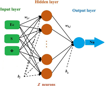
Artificial neural network (ANN) is a computational method for prediction of output solutions in complex systems. ANN, inspired by biological neural systems and human brain, possesses numerous interconnected processing elements called neurons working together harmoniously for solving problems. The multilayer perceptron (MLP) is the most famous and promising ANN among the available ANN models (Cay et al., 2012). MLP network encompasses at least three layers, an input layer, an output layer and one or more hidden layer(s). In MLP network, the number of layers mainly depends on the complexity of problems. Each layer possesses some neurons in which the number of input and output layers is equal to the number of input and output variables. In the current study the number of variables is considered to be 3 and 1. Nevertheless, number of neurons in hidden layer (layers) hasn’t got any specific values which is related to the problem and needs trials for determination. It should be pointed out that the neurons in one layer are connected to the neurons of next layer, but there is no interconnection between neurons at the same layer (Akdag et al., 2016). In this paper, ANN is composed of one input layer, one hidden layer (the number neurons (Z) of hidden layer will be determined) and one output layer illustrated in Figure 2.
The data in input layer’s neurons (input variables received from outside) do not process as the data in the hidden and output layers. It is worth mentioning that outputs are created by summation and activation functions. In these layers, all neuron’s inputs are multiplied by weights and are then aggregated by biases to produce summation functions as follows (Akdag et al., 2016):
| \[\text{Ne}t_{j} = \sum_{i = 1}^{n}{w_{\text{ij}}x_{i} + b_{j}}\] | (14) |
where \(\text{Net}_{j}\) is the summation function of the \(j\)th neuron for the inputs transported from former layer possessing n neurons, \(w_{\text{ij}}\) is the weight between \(j\)th and \(i\)th neurons in pervious layer, \(x_{i}\) is the output of \(i\)th neuron in pervious layer and \(b_{j}\) is the bias term of the \(j\)th neuron. Neurons in hidden and output layers have specific activation function for generation of outputs from summation function. In this paper, hyperbolic tangent sigmoid (tansig) and linear function (purelin) are used as hidden and output layers’ activation function as follows, respectively (Azizi and Ahmadloo, 2016):
| \[\text{Ou}t_{j} = \left\{ \begin{matrix} \frac{e^{\text{Ne}t_{j}} - e^{- \text{Ne}t_{j}}}{e^{\text{Ne}t_{j}} + e^{- \text{Ne}t_{j}}} & ,for\ hidden\ layer\ neurons \\ \text{Ne}t_{j} & ,for\ output\ layer\ neuron \\ \end{matrix}\begin{matrix} \\ \\ \end{matrix} \right.\ \] | (15) |
where \(\text{Out}_{j}\) is the \(j\)th neuron output.
Learning Algorithm
The weights and biases used in summation function need a learning algorithm to determine their values. The learning process, called training, is iterated for adjusting weights and biases until the ANN reaches one of the stopping criteria such as number of epochs, number of validation checks and performance function value. In other words, finding the optimal set of weights and biases is the main goal of the learning process. There are many learning algorithms for training like gradient descent with adaptive learning rule, gradient descent with momentum adaptive learning rule, scaled conjugate gradient and Levenberg-Marquardt (LM) (Cay et al., 2012). In this study, LM was utilized as the training function for learning process due to its fast convergence and stability in training (Azizi and Ahmadloo, 2016).
Training, Validation and Testing Data
The ANN’s input data are classified into three groups called training, validation and testing data. According to the literature, different ratios have been considered for the data set so far (Akdag et al., 2016). A total of 128 numerical data points were selected for ANN considering Eckert number (Ec), squeezing parameter (S) and solid volume fraction (Φ) as input variables and Nusselt number (Nu) as output variable. The percentage of training, validation and testing data were considered as 70%, 15% and 15%, respectively.
Statistical Criteria for Outputs Comparison
Network outputs are compared with actual data obtained from numerical simulation for investigating the performance of the ANN in predicting the solution of the problem. For the ANN, statistical criteria of mean square error (MSE), root mean square error (RMSE), coefficient related to the actual and predicted values (R) and mean relative error (MRE) defined as follows (Azizi and Ahmadloo, 2016):
| \[\text{MSE} = \frac{1}{n}\sum_{m = 1}^{n}\left( Y_{\text{Num},m} - Y_{\Pr\text{ed},m} \right)^{2}\] | (16) |
| \[\text{RMSE} = \sqrt{\frac{1}{n}\sum_{m = 1}^{n}\left( Y_{\text{num},m} - Y_{\Pr\text{ed},m} \right)^{2}}\] | (17) |
| \[R = \sqrt{\left\lbrack \frac{\sum_{m = 1}^{n}\left( Y_{\Pr\text{ed},m} - {\overline{Y}}_{\Pr\text{ed}} \right)\left( Y_{\text{Num},m} - {\overline{Y}}_{\text{Num}} \right)}{\sum_{m = 1}^{n}\left( Y_{\Pr\text{ed},m} - {\overline{Y}}_{\Pr\text{ed}} \right)^{2}\left( Y_{\text{Num},m} - {\overline{Y}}_{\text{Num}} \right)^{2}} \right\rbrack}\] | (18) |
| \[\text{MRE} = \frac{1}{n}\left\lbrack \sum_{m = 1}^{n}\left( \frac{\left| Y_{\text{Num},m} - Y_{\Pr\text{ed},m} \right|}{Y_{\text{Num},m}} \right) \times 100 \right\rbrack\] | (19) |
where \(n\), \(Y_{\text{Num}}\) and \(Y_{\text{Pred}}\) are the number of data points, numerical value and network output, respectively. \({\overline{Y}}_{\text{Num}}\) and \({\overline{Y}}_{\text{Pred}}\) are the average value of \(Y_{\text{Num}}\) and \(Y_{\text{Pred}}\), respectively.
NUMERICAL METHOD
The current problem is a boundary value problem (BVP) and so a proper numerical solver is required. Most of the existing numerical solvers in MAPLE software are achieved based on the combination of trapezoid or midpoint methods. Each of these basic schemes has its own specifications. Methods implemented based on trapezoid method work efficiently for typical problems; however, midpoint-based techniques are highly beneficial for handling harmless end-point singularities. Fourth order Runge–Kutta method is a midpoint approach that improves the Euler method by one order (Sheikholeslami et al., 2012). In this section, the normalized equations (8-9) which are coupled with the boundary conditions given in Eq. (10) are numerically solved by Runge–Kutta method utilizing MAPLE software. Fourth order is the most popular Runge–Kutta methods because the second-order approaches have infinite number of versions. The following formulation is the most commonly used form, i.e. the forth order Runge–Kutta method:
| \[y_{i + 1} = y_{i} + \frac{1}{6}\left( k_{1} + 2k_{2} + 2k_{3} + k_{4} \right)\] | (20) |
where
| \[k_{1} = E\left( x_{i},y_{i} \right)\] | (21) |
| \[k_{2} = E\left( x_{i} + \frac{1}{2}h,y_{i} + \frac{1}{2}k_{1}h \right)\] | (22) |
| \[k_{3} = E\left( x_{i} + \frac{1}{2}h,y_{i} + \frac{1}{2}k_{2}h \right)\] | (23) |
| \[k_{4} = E\left( x_{i} + h,y_{i} + k_{3}h \right)\] | (24) |
It is worth mentioning that the fourth-order Range-Kutta numerical solver is a simple and efficient potential technique for solving differential equations. Table 2 presents the numerical results obtained by Range-Kutta method.
|
Table 2. Numerical results obtained from Runge–Kutta method
|
|||||||||||||||||||||||||||||||||||||||||||||||||||||||||||||||||||||||||||||||||||||||||||||||||||||||||||||||||||||||||||||||||||||||||||||||||||||||||||||||||||||||||||||||||||||||||||||||||||||||||||||||||||||||||||||||||||||||||||||||||||||||||||||||||||||||||||||||||||||||||||||||||||||||||||||||||||||||||||||||||||||||||||||||||||||||||||||||||||||||||||||||||||||||||||||||||||||||||||||||||||||||||||||||||||||||||||||||||||||||||||||||||||||||||||||||||||||||||||||||||||||||||||||||||||||||||||||||||||||||||||||||||||||||||||||||||||||||||||||||||||||||||||||||||||||||||||||||||||||||||||||||||||||||||||||||||||||||||||||||||||||||||||||||||||||||||||||||||||||||||||||||||||||||||||||||||||||||||||||||||||||||||||||||||||||||||||||||||||||||||||||||||||||||||||||||||||||||||||||||||||||||||||||||||||||||||||||||||||||||||||||||||||||||||||||||||||||||||||||||||||||||||||||||||||||||
RESULTS AND DISCUSSION
Results of Neural Network
In this study, Matlab software was employed for coding ANN computer program. The ANN was used for different neuron numbers in hidden layer varying from 1 to 20. In order to reach hidden layer’s optimum neuron number, the number of runs was set to be 50. The performance of each network is presented in Table 3. According to the results, the network with 16 neurons in hidden layer (3-16-1) has the best performance for which RMSE is found to be 0.001364 for testing data. Furthermore, the network possesses the best MRE and R whose values are found to be 0.033837% and 1, respectively.
|
Table 3. Performance results of testing data obtained from ANN for hidden layer with different neuron numbers
|
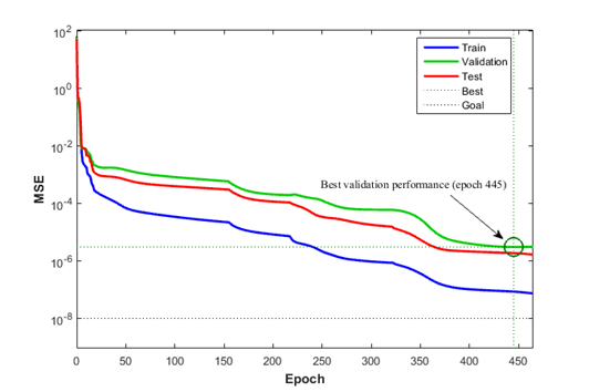
Figure 3 indicates the variation of MSE with epoch during training process for reaching optimum network (3-16-1) in which the minimum MSE of validated data is found to be of \(3.0342 \times 10^{- 6}\) occurring at epoch 445.
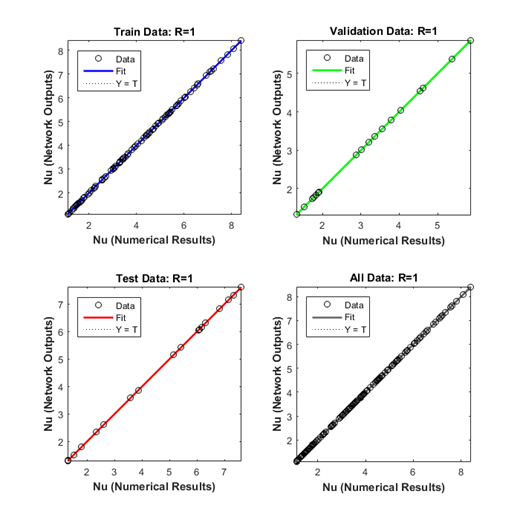
The numerical results versus the predicted values are presented in Figure 4 for the training, validation, testing and all data sets for which R is equal to unity showing the highest accuracy of the network prediction. The performance of each data set is given in Table 4 based on the RMSE, R, MRE. The training data set has the best performance and the performance of testing data set is better than that of validation data set.
|
Table 4. Performance of ANN for training, validation and testing data sets
|
|||||||||||||||||||||||||||||||||
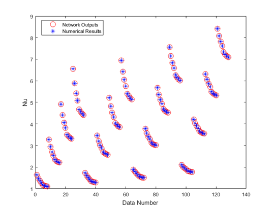
Figure 5 compares the numerical results and the network prediction values for all data sets. As can be seen in this figure, there is an appropriate agreement between the numerical and network predicted results. Thus, the network is efficiently capable of predicting Nusslet number in this problem.
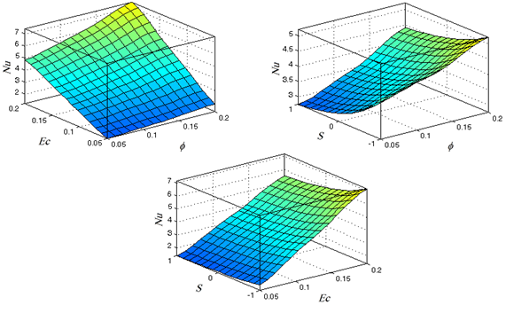
Influences of solid volume fraction, moving parameter and Eckert number on Nusselt number are depicted in Figures 6(a)-6(c). As can be implied from Figure 6(a), for constant values of moving parameter, when the Eckert number is lower than or equal to 0.05, an increment in nanoparticle volume fraction leads to significant changes in thermal boundary layer thickness and value of Nusselt number. Nevertheless, at high values of Eckert number, an increase in nanoparticles volume fraction results in more intensive growth in thermal boundary layer thickness and greater values of Nusselt number are obtained.
With regard to Figure 6(b), impact of moving parameter on Nusselt number is more crucial than solid volume fraction. As already expressed, taking into account constant values of Eckert number and solid volume fraction, the maximum value of Nusselt number occurs when \(S = - 1\).
It is notable that an enhancement in the absolute magnitude of moving parameter is directly related to kinematic viscosity reduction and increment of moving speed of the plates, which causes faster growth of thermal boundary layer and higher values of Nusselt number. Regarding Figure 6(b), this value (Nusselt number) will be increase by increment of\(\varphi\).
Figure 6(c) depicts the impact of Eckert number and moving parameter on Nusselt number. According to this figure, it is obvious that the moving parameter plays key role in heat transfer performance and its effect on Nusselt number is significant. As can be observed in Figure 6(c), changing the value of moving parameter from 0 to -1 leads to an increment in Nusselt number from to 1.3 to 1.6. This effect is more intensive at higher values of Eckert number. Also it can be implied that raising the value of Eckert number results in enhancement in the surface curvature when solid particle volume fraction is constant.
CONCLUSION
In the present paper, heat transfer in a two-dimensional unsteady nanofluid flow between two parallel moving plates was studied applying artificial neural network. In order to present reliable results, a powerful numerical method known as forth order Runge-Kutta method was employed for solving the coupled nonlinear ordinary differential governing equations. Subsequently, the results yielded by ANN were compared with the numerical results. On the basis of the results, it was revealed that an increment in the absolute magnitude of moving parameter was directly affected by kinematic viscosity reduction and increment of plates moving speed. Moreover, increase in the moving parameter caused faster growth in thermal boundary layer and a remarkable increase in the value of Nusselt number.
Nomenclature
| \[u\] | Velocity in x direction |
| \[v\] | Velocity in y direction |
| \[p\] | Pressure |
| \[\rho_{\text{nf}}\] | Effective density of nanofluid |
| \[{{(\rho C}_{P})}_{\text{nf}}\] | Effective heat capacity of nanofluid |
| \[k_{\text{nf}}\] | Effective thermal conductivity of nanofluid |
|
Nu |
Nusselt Number |
| \[\Pr\] | Prandtl number |
| \[S\] | Moving parameter |
Greek symbols |
|
| \[\alpha\] | Constant rotational velocity |
| \[\varphi\] | Dimensionless concentration |
| \[\mu\] | Dynamic viscosity |
| \[\vartheta\] | Kinematic viscosity |
| \[\theta\] | Dimensionless temperature |
| \[\rho\] | Fluid density |
Subscripts |
|
| \[f\] | Base fluid |
| \[\text{nf}\] | Nanofluid |
| \[p\] | Nano particle |
References
- Akdag, U., Komur, M. A. and Akcay, S. (2016). Prediction of heat transfer on a flat plate subjected to a transversely pulsating jet using artificial neural networks. Applied Thermal Engineering, 100, 412-420. https://doi.org/10.1016/j.applthermaleng.2016.01.147
- Azimi, M., Azimi, A. and Mirzaei, M. (2014). Investigation of the unsteady Graphene oxide nanofluid flow between two moving plates. Journal of Computational and Theoretical Nanoscience, 11(10), 2104-2109. https://doi.org/10.1166/jctn.2014.3612
- Azimi, M., Azimi, A. and Mirzaei, M. (2015). Analytical Investigation of MHD Jeffery Hamel Problem with Graphene Oxide Nanoparticles using GOHAM. Journal of Computational and Theoretical Nanoscience, 12(6), 991-995. https://doi.org/10.1166/jctn.2015.3839
- Azimi, M. and Riazi, R. (2015). Heat transfer analysis of GO-water nanofluid flow between two parallel disks. Propulsion and Power Research, 4, 23-30. https://doi.org/10.1016/j.jppr.2015.02.001
- Azimi, M. and Mozaffari, A. (2015). Heat transfer analysis of unsteady graphene oxide nanofluid flow using a fuzzy identifier evolved by genetically encoded mutable smart bee algorithm. Engineering Science and Technology, an International Journal, 18(1), 106-123. https://doi.org/10.1016/j.jestch.2014.10.002
- Azizi, S. and Ahmadloo, E. (2016). Prediction of heat transfer coefficient during condensation of R134a in inclined tubes using artificial neural network. Applied Thermal Engineering, 106, 203-210. https://doi.org/10.1016/j.applthermaleng.2016.05.189
- Cay, Y., Cicek, A., Kara, F. and Sagiroglu, S. (2012). Prediction of engine performance for an alternative fuel using artificial neural network. Applied Thermal Engineering, 37, 217-225. https://doi.org/10.1016/j.applthermaleng.2011.11.019
- Eiamsa-ard, S. and Changcharoen, W. (2015). Flow structure and heat transfer in a square duct fitted with dual/quadruple twisted-tapes: Influence of tape configuration. Journal of Mechanical Science and Technology, 29(8), 3501-3518. https://doi.org/10.1007/s12206-015-0748-z
- Hamad, M. A. A., Pop, I. and MdIsmail, A. I. (2011). Magnetic field effects on free convection flow of a nanofluid past a vertical semi-infinite flat plate. Nonlinear Analysis: Real World Applications, 12, 1338–1346. https://doi.org/10.1016/j.nonrwa.2010.09.014
- Jianu, O. A. and Rosen, M. A. (2017). Preliminary Assessment of Noise Pollution Prevention in Wind Turbines Based on an Exergy Approach. European Journal of Sustainable Development Research, 1(2), 12. https://doi.org/10.20897/ejosdr.201712
- Kim. Y. C. (2014). Effect of surface roughness on pool boiling heat transfer in subcooled water-CuO nanofluid. Journal of Mechanical Science and Technology, 28(8), 3371-3376. https://doi.org/10.1007/s12206-014-0749-3
- Kumar, P. C. M., Palanisamy, K., Kumar, J., Tamilarasan, R. and Sendhilnathan, S. (2015). CFD analysis of heat transfer and pressure drop in helically coiled heat exchangers using Al2O3/water nanofluid. Journal of Mechanical Science and Technology, 29(2), 697-705. https://doi.org/10.1007/s12206-015-0129-7
- Kumar, P. C. M., Kumar, J., Tamilarasan, R., Nathan. S. S. and Suresh, S. (2014). Heat transfer enhancement and pressure drop analysis in a helically coiled tube using Al2O3 / water nanofluid. Journal of Mechanical Science and Technology, 28(5), 1841-1847. https://doi.org/10.1007/s12206-014-0331-z
- Lihong, Y. and Hangming, S. (2015). Study on thin copper-wire distribution for heat transfer enhancement from wall to interior of an isothermal chamber. Journal of Mechanical Science and Technology, 29(4), 1377-1382. https://doi.org/10.1007/s12206-015-0307-7
- Moslehi, M. and Saghafian, M. (2015). MHD mixed convection slip flow in a vertical parallel plate microchannel heated at asymmetric and uniform heat flux. Journal of Mechanical Science and Technology, 29(12), 5317-5322. https://doi.org/10.1007/s12206-015-0739-0
- Muthtamilselvan, M., Prakash, D. and Doh, D. H. (2014). Effect of thermal non-equilibrium on transient hydromagnetic flow over a moving surface in a nanofluid saturated porous media, Journal of Mechanical Science and Technology, 28(9), 3709-3718. https://doi.org/10.1007/s12206-014-0832-9
- Rahimi-Gorji, M., Pourmehran, O., Gorji-Bandpy, M. and Ganji, D. D. (2016). Unsteady squeezing nanofluid simulation and investigation of its effect on important heat transfer parameters in presence of magnetic field. Journal of the Taiwan Institute of Chemical Engineers, 67, 467-475. https://doi.org/10.1016/j.jtice.2016.08.001
- Shahriari, G., Maghsoudi, P. and Sadeghi, S. (2018). Impact of Viscous Dissipation on Temperature Distribution of a Two-dimensional Unsteady Graphene Oxide Nanofluid Flow between Two Moving Parallel Plates Employing Akbari-Ganji Method. European Journal of Sustainable Development Research, 2(2), 24. https://doi.org/10.20897/ejosdr/81574
- Sheikholeslami, M., Ashorynejad, H. R., Domairry, G. and Hashim, I. (2012). Flow and Heat Transfer of Cu-Water Nanofluid between a Stretching Sheet and a Porous Surface in a Rotating System. Journal of Applied Mathematics, 35, 1-20. https://doi.org/10.1155/2012/421320
- Sheikholeslami, M., Soleimani, S., Gorji-Bandpy, M., Ganji, D. D. and Seyyedi, S. M. (2012). Natural convection of nanofluids in an enclosure between a circular and a sinusoidal cylinder in the presence of magnetic field. International Communications in Heat and Mass Transfer, 39(9), 1435-1443. https://doi.org/10.1016/j.icheatmasstransfer.2012.07.026
- Sheikholeslami, M., Ganji, D. D. and Ashorynejad, H. R. (2013). Investigation of squeezing unsteady nanofluid flow using ADM. Powder Technology, 239, 259-265. https://doi.org/10.1016/j.powtec.2013.02.006
- Sheikholeslami, M. and Ganji, D. D. (2013). Heat transfer of Cu-water nanofluid flow between parallel plates. Powder Technology, 235, 873-879. https://doi.org/10.1016/j.powtec.2012.11.030
How to cite this article
APA
Gorgani, H. H., Maghsoudi, P., & Sadeghi, S. (2019). An Innovative Approach for Study of Thermal Behavior of an Unsteady Nanofluid Squeezing Flow between Two Parallel Plates Utilizing Artificial Neural Network. European Journal of Sustainable Development Research, 3(1), em0069. https://doi.org/10.20897/ejosdr/3935
Vancouver
Gorgani HH, Maghsoudi P, Sadeghi S. An Innovative Approach for Study of Thermal Behavior of an Unsteady Nanofluid Squeezing Flow between Two Parallel Plates Utilizing Artificial Neural Network. EUR J SUSTAIN DEV RES. 2019;3(1):em0069. https://doi.org/10.20897/ejosdr/3935
AMA
Gorgani HH, Maghsoudi P, Sadeghi S. An Innovative Approach for Study of Thermal Behavior of an Unsteady Nanofluid Squeezing Flow between Two Parallel Plates Utilizing Artificial Neural Network. EUR J SUSTAIN DEV RES. 2019;3(1), em0069. https://doi.org/10.20897/ejosdr/3935
Chicago
Gorgani, Hamid Haghshenas, Peyman Maghsoudi, and Sadegh Sadeghi. "An Innovative Approach for Study of Thermal Behavior of an Unsteady Nanofluid Squeezing Flow between Two Parallel Plates Utilizing Artificial Neural Network". European Journal of Sustainable Development Research 2019 3 no. 1 (2019): em0069. https://doi.org/10.20897/ejosdr/3935
Harvard
Gorgani, H. H., Maghsoudi, P., and Sadeghi, S. (2019). An Innovative Approach for Study of Thermal Behavior of an Unsteady Nanofluid Squeezing Flow between Two Parallel Plates Utilizing Artificial Neural Network. European Journal of Sustainable Development Research, 3(1), em0069. https://doi.org/10.20897/ejosdr/3935
MLA
Gorgani, Hamid Haghshenas et al. "An Innovative Approach for Study of Thermal Behavior of an Unsteady Nanofluid Squeezing Flow between Two Parallel Plates Utilizing Artificial Neural Network". European Journal of Sustainable Development Research, vol. 3, no. 1, 2019, em0069. https://doi.org/10.20897/ejosdr/3935

 Full Text (PDF)