Abstract
To help balance comfort and energy use in residential, institutional and commercial buildings in order to make them more sustainable, a thermal comfort model is coupled with a computational fluid dynamic approach. The developed tool provides an effective tool for demand side management of energy use in buildings. The asymmetrical thermal environment in a university cafeteria building is modeled, and a two dimensional numerical simulation is prepared separately of the thermal sensation in the cafeteria. A finite volume formulation is used to provide the temperature distribution around a space-variant manikin, which is in turn utilized to determine the convective heat transfer coefficients for the simulation of thermal sensation around the manikin.
License
This is an open access article distributed under the Creative Commons Attribution License which permits unrestricted use, distribution, and reproduction in any medium, provided the original work is properly cited.
Article Type: Research Article
EUR J SUSTAIN DEV RES, Volume 2, Issue 1, 2018, Article No: 07
https://doi.org/10.20897/ejosdr/63225
Publication date: 30 Jan 2018
Article Views: 3683
Article Downloads: 2188
Open Access HTML Content References How to cite this articleHTML Content
INTRODUCTION
The thermal load of a building has two main parts: heating and cooling. These loads are managed by adding or removing heat, and this is accomplished with heating, ventilating and air conditioning (HVAC) systems.
Normally, the indoor environment of a building is designed to satisfy human physiological needs, as well as other needs like psychological and physical requirements (Djongyang et al., 2010). Efforts to develop or select efficient HVAC systems often do not address successfully any dissatisfaction people have with the indoor thermal conditions, affecting the sustainability of the building. Dissatisfaction can derive from deficiencies in energy supply or other factors. Providing thermal comfort is responsible for a significant portion of the energy consumption of a typical building, but energy use affects the natural environment including ecological systems. Therefore, an appropriate trade off in optimum building design between energy efficiency and indoor thermal comfort is needed for sustainable buildings, but this trade off is not well understood.
Nevertheless, some efforts have been made to address this issue, at least preliminarily. A consumption-driven incentive approach was applied by Ogedengbe et al. (2011), in studying the energy demands of residential buildings in Ontario, Canada. By considering the analysis of the demands several cooling and heating appliances, including hot-water tanks and electric/gas furnaces, in both residential and commercial stocks for major cities in the province of Ontario, it was shown that the control and management of thermal comfort and indoor air quality accounts for more than 47% of the total energy demand, on average. This North American trend is consistent with the patterns of energy demand for thermal comfort in residential and commercial buildings in such European countries as Italy (Caldera et al., 2008; Schiavon and Melikov, 2008) and Norway (Satori et al., 2009), and in Asia (Homod et al., 2012).
The adaptive approach uses historical energy usage data for building stock, the energy balance approach, and is described well by Fanger (1970). Another approach is based on data from climate chamber studies (Ogedengbe et al., 2013). Fanger’s (1972) experimentally derived comfort equation obtains the predicted percentage dissatisfied (PPD) for people in an indoor climate, as a meaningful measure. PPD is obtained using the predicted mean vote (PMV) for several positions in a room. The PMV model is the most commonly used method in practice presently for predicting the thermal comfort/discomfort in a building design and for assessing the discomfort in existing building environments.
Several researchers have investigated the capabilities of thermal comfort models, including Cheng et al. (2012) who proposed the sustainable advantage of a computational fluid dynamics approach for the simulation of thermal sensation in asymmetrical environments. These thermal comfort models are generally classified into physiological comfort models (which predict the thermal sensation of the body physiology), and psychological comfort models (which depend on accurate prediction of the thermal environments). Accurate modelling of thermal comfort depends on several factors, including a reliable prediction of the nature of the asymmetrical environment, the variation in the level of thermal sensation for various parts of human body, and the stability and accuracy of the adopted CFD platform (Arens, 2006). Gao et al. (2007) adopted the Berkeley thermal comfort model, and coupled several subsystems, including the displacement ventilation (DV), mixing ventilation (MV) and personalized ventilation (PV) subsystems, in a CFD environment to assess human thermal comfort. The heat transfer between the human body and the environment was demonstrated to be complicated. Several other researchers in these two fields have attempted to develop reliable human thermal physiological models. These vary from simple one-node models to complex three-dimensional finite element models (Djongyang, 2010; Carlucci and Pagliano, 2012).
The US Energy Information Administration (EIA) reported that buildings represent a major source of global energy consumption and greenhouse gas (GHG) emissions. In 2001, annual energy consumption and GHG emissions accounted for 48% of the total residential energy consumption, broken down as energy used by residential buildings for space heating (46.7%) and cooling (6.5%) (EIA, 2001). Unfortunately, demand side monitoring to improve heating and cooling efficiency in residential building does not easily attract the investment of effort and time on CFD tools, mainly due to unclear economic arguments.
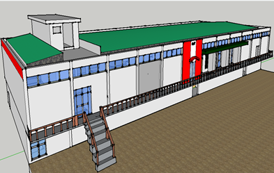
In this paper, we seek to address these issues and help enhance building sustainability. The research reported here attempts the deployment of a two-dimensional finite volume formulation of an environment constituted by the 2001 Cafeteria of the University of Lagos (see Figure 1).
FINITE VOLUME FORMULATION
The main hall of the 2001 Campus Cafeteria is the asymmetrical environment, which is subjected to thermal comfort analysis. Thermal comfort modeling is coupled with comparative computation of convective heat transfer from a space variant manikin in order to assess the energy demand of the building environment. Depending on the adopted implementation platform, the boundary conditions are imposed on the built environment in order with the analysis of the relevant physiological and environmental data.
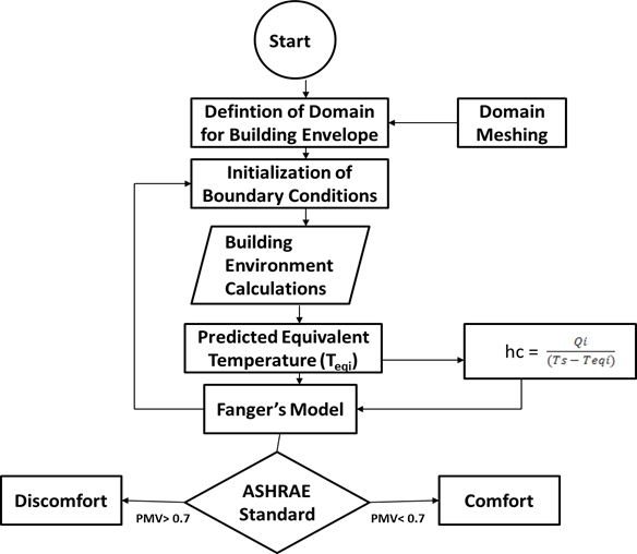
A flow chart for the computation of thermal comfort is shown in Figure 2. Human thermal sensation varies spatially in an asymmetrical environment. With different environmental parameters around the manikin, including velocity and temperature, the thermal sensation variables can be evaluated with CFD based on specified boundary conditions. The depicted CFD solution procedure, incorporating the algorithm for simulating the thermal sensations around the manikin, represents a significant part of the methodology for thermal comfort analysis. A significant contribution of the proposed solution procedure involves the determination of the equivalent temperature and convective heat transfer coefficient of body parts, which are coupled with Fanger’s model in order to estimate the thermal sensation of the body segments. Treating the movement of room air with the building envelope as a continuum, thermal sensations may be determined by solving the discretized mass, momentum, and energy equations, with specified boundary conditions. Considering the dynamics of natural convection within the context of building simulation, the Boussinesq approximation is applied, whereby air density is fixed and buoyancy effects are accounted for in the momentum equation (Ogedengbe, 2006; Ogedengbe and Naterer, 2004):
| \[\frac{\partial(\rho)}{\partial t} + \frac{\partial(\rho u)}{\partial x} + \frac{\partial(\rho v)}{\partial y} = 0\] | (1) |
| \[\frac{\partial(\text{ρU})}{\partial t} + \nabla \cdot (\text{ρvU}) = - \frac{\partial P}{\partial x} + \nabla \cdot (\mu\nabla U) + {\dot{S}}_{U}\] | (2) |
| \[\frac{\partial(\text{ρV})}{\partial t} + \nabla \cdot (\text{ρvV}) = - \frac{\partial P}{\partial y} + \nabla \cdot (\mu\nabla V) + {\dot{S}}_{V}\] | (3) |
| \[\frac{\partial(\rho c_{p}T)}{\partial t} + \nabla \cdot (\rho c_{p}\text{vT}) = \nabla \cdot (k\nabla T)\] | (4) |
Here, the buoyancy terms are
| \[{\dot{S}}_{U} = \rho_{\infty}B_{\infty}g_{x}\left( T_{P} - T_{\infty} \right)\] | (5) |
| \[{\dot{S}}_{V} = \rho_{\infty}B_{\infty}g_{y}\left( T_{P} - T_{\infty} \right)\] | (6) |
The Grashof, Prandtl and Raleigh numbers are expressed as \(G_{r} = \ \rho^{2}gB\mathrm{\Delta}TL^{3}/\mu^{2}\), \(P_{r} = \ \mu c_{p}/k\) and \(R_{a} = G_{r}P_{r}\), respectively. The Grashof and Raleigh numbers represent relevant dimensionless parameters related to natural convection, which are incorporated in the models for building envelopes of typical residential and commercial systems.
The two-dimensional plane for the CFD analysis of the building envelope is carefully selected in order to ensure that the asymmetrical environment is sufficiently captured. For the selected plane and given boundary configurations, numerical methods are employed to determine the temperature distribution within the building envelope. We combine the use of CFD tools with available building energy performance models, using various numerical formulations (e.g., finite element and finite volume). The finite volume method has proven more successful at conserving mass than the finite element method (Ogedengbe, 2006), so a finite volume platform is adopted here in developing the numerical model for the fluid flow and thermal sensations in the considered cafeteria.
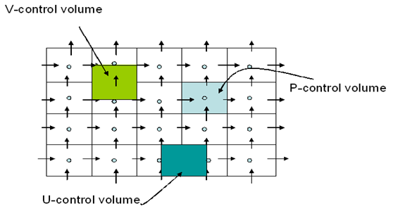
A standard finite volume procedure is adopted, utilizing the conventional SIMPLEC algorithm. Figure 3 depicts a typical staggered grid in a 2-D finite volume formulation. Note that advection is incorporated with a new convection formulation using mass-weighted interpolation of upstream convection variables. This Non-Inverted Skew Upwind Scheme (formulation accommodates flow directionality dependences, and exhibits reasonable accuracy and stability (Ogedengbe and Naterer, 2004).
A staggered grid arrangement is adopted for the SIMPLEC formulation (see Figure 3), where separate U- and V- control volumes are employed for the momentum equations. The pressure control volume (or scalar control volume) is located at the center node of the discretized domain, while the velocity control volumes (i.e., either the U- control volumes or the V- control volumes) are adjacent. The net flows across a control volume boundary are the sum of the integrated flux terms for the four control volume edges, following Equations (1) to (4). The scalar conservation equation is represented as follows (Ogedengbe, 2006; Ogedengbe and Naterer, 2004):
| \[a_{p}\phi_{p} = \sum_{}^{}{a_{\text{nb}}\phi_{\text{nb}} + b}\] | (7) |
Here, \(a\), \(\phi\) and \(b\) denote respectively finite volume coefficient, scalar variable (e.g., velocity component, temperature) and source term, while subscripts \(p\) and \(\text{nb}\) denote respectively central and neighboring nodes.
The accuracy of the flow simulation depends largely on the stability of the upwind scheme that is used for the approximation of the advection of field variables. The SIMPLEC algorithm uses the exponential scheme with slight weighting on Non-Inverted Skew Upwind Scheme for coupling the advection terms in the governing equations. Ogedengbe (Ogedengbe, 2006) reported a detailed numerical formulation of the pressure-velocity correction algorithm and the approximation of the upwind scalar values from the Non-Inverted Skew Upwind. With the solutions, the rate of change of any scalar property can be determined based on the discretized form of equation (7). The discretized form of the steady transport equation of property \(\phi\) is:
| \[{\dot{m}}_{e}\phi_{e} - {\dot{m}}_{w}\phi_{w} + {\dot{m}}_{n}\phi_{n} - {\dot{m}}_{s}\phi_{s} + \Gamma_{e}A_{e}\left\lbrack \frac{\text{dϕ}}{\text{dx}} \right\rbrack_{e} - \Gamma_{w}A_{w}\left\lbrack \frac{\text{dϕ}}{\text{dx}} \right\rbrack_{w} + \Gamma_{n}A_{n}\left\lbrack \frac{\text{dϕ}}{\text{dy}} \right\rbrack_{n} - \Gamma_{s}A_{s}\left\lbrack \frac{\text{dϕ}}{\text{dy}} \right\rbrack_{s} = \widehat{S}\Delta V\] | (8) |
where \(\mathrm{\Delta}x\) and \(\mathrm{\Delta}y\) are grid spacing in the \(x\) and \(y\) directions respectively, and \(\mathrm{\Delta}V\) is the flow domain volume.
The building energy management system (BEMS) field integrates various disciplines in engineering and the sciences, including applied physics, communications, networking, cloud computing, material science, applied mechanics, thermodynamics, system engineering, and management. Considering the dearth of environmental data in most software packages developed for load analysis in building envelopes, determining a best methodology for effective building management, including optimization of insulation thickness and the determination of the minimum energy performance standards for the appliances, is challenging (Gao et al., 2007). Comprehensive energy audit procedures for the development of a reliable BEMS result in two data gathering categories. The first category includes instruments for metering parameters like air velocity, indoor temperature, relative humidity, etc. The second incorporates sensors with building devices (Ogedengbe et al., 2012).
Effective forecasting of the building energy demand is helpful for the design of a sustainable building energy system. For instance, Ogedengbe et al. (2014) recently proposed the possibility of developing an organic photovoltaic solar technology based on the data gathered from an audit of the entire Faculty of Engineering in the University of Lagos.
NUMERICAL SIMULATION
Consider a manikin seated in the flow domain. The simulation domain is composed of the surrounding air (which is characterized by its density \(\rho = 1.161\ kg/m^{3}\) thermal conductivity \(k = 0.0263\ \text{W\ }m^{- 1}\ K^{- 1}\), specific heat capacity \(C_{p} = 1.007\ \text{J\ k}g^{- 1}\ K^{- 1}\) and dynamic viscosity \(\mu = 1.827 \times \ 10^{- 5}\ kg/(ms)\)). For the selected plane of the computation domain, the boundary conditions imposed are based on the measured environmental data for the 2001 cafeteria (see Table 1).
|
Table 1. Built Environment Boundary Conditions
|
||||||||||||||||||||||||||||||||||||||||
|
Table 2. Physiological Data for Assessing Convective Heat Emission of Body Segments
|
The thermal sensation experiment depends on the combination of the physiological data of the manikin and the environmental data. Basic body parameters, as used in this study, are similar to those for the model designed at Kansas State University by Fu (Fanger, 1972), for the examination of the basal metabolic generation. Table 2 shows the physiological data of a typical manikin, including the length of the body cylindrical segment (m) and the corresponding heat flux, which is based on other studies (Schellen, 2013). The solution algorithm in Figure 2 yields the required field variables for the calculation of the predictive data for the thermal sensation experiment. The equivalent temperature is obtained from the simulated air velocity and operative temperature. But the temperature of the skin surface is assumed constant, based on ASHRAE standards as defined subsequently by Equation (17) (ASHRAE, 1997).
Radiation effects appear negligible in most simulations of thermal sensations of people in building environments. But where it is relevant, Loomans (1998) proposed a simplified approach for the treatment of the interactions with the skin, where radiation effects are accounted for in the convective portion of the heat emission from people (52% of 112 W). The heat emissions from body parts are calculated proportionally according to the surface area of the arteries and veins in each segment (Salloum et al., 2007). This approach is inconsistent with that of Schellen et al. (2013), which applies the segment area to determine the segment heat flux. A simplified geometrical shape is used to approximate the shape of different of the body segment. For example, the head can be a sphere while the neck takes the shape of a cylinder. We treat arteries and veins as cylinders, for which the surface area is \(2\pi rl\). Then the surface area of an artery or vein segment \(S_{a,v}\) can be written as follows:
| \[S_{a,v} = 2\pi\left( r_{a} + r_{v} \right)l_{i}\] | (9) |
Here, \(r_{a}\) is the artery radius in the body segment, \(r_{v}\) the vein radius in the body segment, and \(l_{i}\) the body segment length. The quantity \(2\pi\left( r_{a} + r_{v} \right)\) is constant for all segments, leaving the length of the surface \(l_{i}\) as the basis for proportional determination of the convective heat emission for body parts.
Various values have been reported for the convective heat transfer coefficients for body parts (Schellen et al., 2013; Fiala, 1998; De Dear et al., 1997). The heat transfer coefficient is assumed to be linearly relatied to heat flux and to temperature difference (Najjaran, 2012; Kurazumi et al., 2008).
|
Table 3. Comparison of Convective Heat Transfer Coefficient, \(\mathbf{h}_{\mathbf{c}}\), for Body Parts with Results of Schellen (2013)
|
|||||||||||||||||||||||||||||||||||||||||||
|
Table 4. Comparison of Convective Heat Transfer Coefficient, \(\mathbf{h}_{\mathbf{c}}\), for Body Parts with the Results of Fiala (1998)
|
|||||||||||||||||||||||||||||||||||||||||||
The convective heat transfer coefficient \(h_{c}\) of a body part can be expressed as:
| \(h_{c} = \frac{Q_{i}}{(T_{s}\ - T_{\text{eqi}})}\) | (10) |
Here, \(h_{c}\) denotes the convective heat transfer coefficient (W/m2 K), \(Q_{i}\) the convective heat emission rate (W/m2), \(T_{s}\) the surface temperature (K), and \(T_{\text{eqi}}\) the average equivalent temperature (K), all for the body segment. The body part surface temperature can be expressed as follows:
| \[T_{s} = 35.7-0.0275(M\ -\ W)\] | (11) |
Here, \(M\) is the metabolic rate and \(W\) the external mechanical work done. The equivalent temperature, obtained with CFD for each body part, is utilized to compute the convective heat transfer coefficient, and an input to Engineering Equation Solver (EES) and. Values are compared in Tables 3 - 4 and Figure 4 for two positions, one obtained here and two obtained by Schellen (2013) and Fiala (1998).
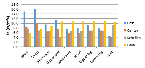
The convective heat transfer coefficient values are used to assess the thermal comfort in the cafeteria. To validate the present results, especially the convective heat transfer coefficient for the positions considered, comparisons are made with related work reported by others. Specifically, Fanger’s model is used for thermal comfort evaluation and Rohles’ (1973) equation is employed for validation.
Fanger’s PMV equation for thermal comfort predicts empirically the mean vote on an ordinal rating scale of thermal comfort of a population, based on a steady-state heat balance for the human body (Thermal Comfort Models, 2018). The equation presumes the deviation from the minimum load on mechanisms affecting the heat balance (sweating, vasoconstriction, vasodilation, etc.) is related to thermal comfort vote. The smaller is the load, the less the comfort vote deviates from zero. The ASHRAE thermal scale utilized is shown by Table 5. The \(\text{PMV}\) can be expressed as
| \[PMV = (0.028 + 0.3033\exp\left( -0.036M \right))L\] | (12) |
and the \(\text{PPD}\) as:
| \[PPD = 100 - 95\exp\left( - 0.03353\ PMV^{4} - \ 0.2179\ PMV^{2} \right)\] | (13) |
Rohles and Nevins (1971) and Rohles (1973) examined 1600 school age students to correlate level of comfort with temperature, humidity, gender and exposure duration, for an air speed below 0.17 m/s, and developed the following expression for \(\text{PMV}\):
| \[PMV = a\left( T_{a} \right) + b\left( P_{a} \right) - c\] | (14) |
where \(a\), \(b\) and \(c\) are empirical coefficients. For the present conditions which are described elsewhere (ASHRAE, 1997; Rohles, 1973), it is reported that \(a = 0.245\), \(b = 0.248\) and \(c = 6.475\).
|
Table 5. PMV Thermal Sensation Scale/Index*
* Based on definitions in (ASHRAE, 1997). |
RESULTS AND DISCUSSION
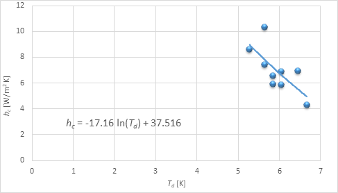
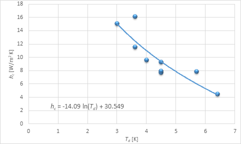
The developed CFD tool is used to determine the equivalent temperature by coupling the air velocity with temperature. The convective heat transfer coefficient for each segment is obtained for the two positions considered. Table 3 provides the convective heat transfer coefficients from this study as well as those reported by Schellen et al. (2013), while Table 4 provides the convective heat transfer coefficients from this study and those obtained by Fiala (1998). The convective heat transfer coefficient is plotted in Figures 5-6 versus the difference between the skin surface temperature and average equivalent temperature for each segment. Thus, the relation between \(h_{c}\) and temperature difference is given in Figure 5 for the manikin at the centre of the domain and in Figure 6 for the manikin located 1.8 m from the wall. The equations for the convective heat transfer coefficient of the body are included in these figures. But predictions that better agree with the simulated results are found to be provided by Equation (16), shown subsequently.
Figures 7 and 8 provide the PMV when the manikin is at the center of the domain and located 1.8 from the east wall, respectively. The maximum deviation occurs at the chest, and has a magnitude of 0.25. Respiration heat loss for the chest by convection, which Salloum et al. (2007) indicates to be significant, is not considered in the determination of the heat flux of that segment. This simplification may cause the deviation for that body segment, but respiration heat loss is negligible for other body segments.
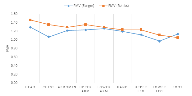
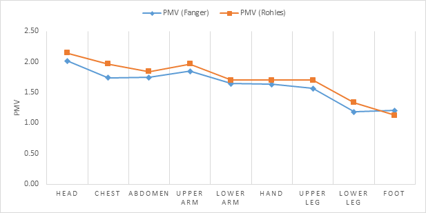
Figures 7 and 8 agree well with Fanger’s model, which is a function of convective heat transfer coefficient \(h_{c}\), and with Rohles equation. The latter is independent of \(h_{c}\) based on Equation (14).
Users of 2001 Cafeteria likely experience some discomfort, due to the differences observed when the results are compared with the ASHRAE thermal sensation scale in Table 5 and the acceptable thermal environment classes for general comfort in Table 6.
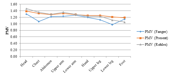
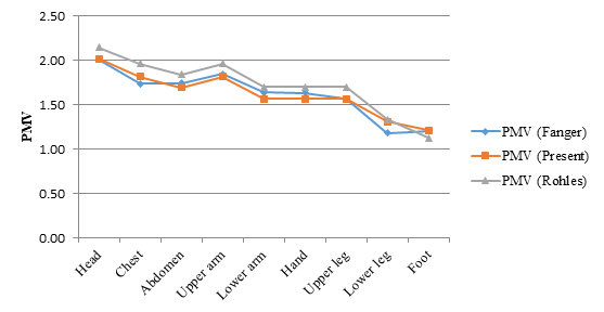
The difference between the PMV obtained with Fanger’s model and Rohles’ model are seen Figures 9 and 10 to be within ±0.28 scale units for both positions considered. Rohles’ equation provides a nearly similar prediction of thermal sensation, providing a beneficial application for building design and thermal comfort analysis, due to its ease of use. Fanger’s comfort equation is however, too complicated to be solved via a simple, manual procedure, it nonetheless provides a detailed analysis that relates variables relevant to thermal sensation prediction. The characteristic curves in Figures 5a and 5b are consistent with the expected thermal sensation of the manikin and the temperature difference within the asymmetrical building environment. These curves can be written as follows. The convective heat transfer coefficient for the manikin at the centre of the domain \(h_{c,c}\) can be expressed as
| \[h_{c,c} = - 17.16\ln T_{d} + 37.516\] | (15) |
and the convective heat transfer coefficient for the manikin located 1.8 m from the east wall hc,w as
| \[h_{c,w} = - 14.09\ln T_{d} + 30.549\] | (16) |
Here,
| \[T_{d} = T_{s} - T_{\text{eq}}\] | (17) |
With Equation (16) developed here, Fanger’s model takes on the following form:
| \[PMV = \left( 0.028 + 0.3033\exp\left( - 0.036M \right) \right)\left\{ \left( M - W \right) - 3.05\left( 5.73 - 0.00699\left( M - W \right) - P_{a} \right) - 0.42\left( \left( M - W \right) - 58.15 \right) - 0.0173M\left( 5.87 - P_{a} \right) - 0.0014M\left( 34 - T_{a} - {3.9610}^{- 8}F_{\text{cl}}\left( \left( T_{\text{cl}} + 273 \right)^{4} - \left( T_{r} + 273 \right)^{4} \right) - F_{\text{cl}}\left\lbrack - 14.09\ln{\left( T_{d} \right) + 30.549} \right\rbrack\left( T_{\text{cl}} - T_{a} \right) \right) \right\}\] | (18) |
Figures 8 and 9 show that the expression for PMV developed here (see Equation (23)) has a deviation of less than ±0.248 scale units from the results obtained with Fanger’s PMV expression (Equation (12)). However, the deviation declines to less than ±0.15 for the two positions considered when the result of the developed model is compared with Rohles model, suggesting that the model developed here reasonably accurately describe the thermal sensation of the domain.
|
Table 6. Three Classes of Acceptable Thermal Environment for General Comfort*
* Based on definitions in (ASHRAE, 1997). |
Elsewhere (Ogedengbe et al., 2013), the Eatery hall of the university is shown to produces 245 kg/day of food waste while other shops within the complex generate 75 kg/day of food waste. Mansour (2010) estimates that 10 kg of kitchen waste produces 1.5 m3 of biogas which consists of 1 m3 of methane. It is therefore estimated that 200 m3 of methane can be generated monthly from the 2001 Cafeteria Complex. Such activity may emit heat and affect thermal comfort.
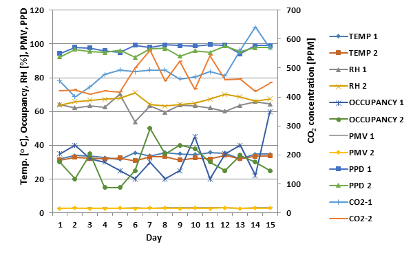
Table 7 lists for various compartments in the cafeteria building several thermophysical properties: orientation, area, thickness, thermal conductivity \(k\). The cafeteria building compartments include the following: Hommies bakery, Unilag Water, Husky Food, Eatery Hall, Wisdom Café, Pinto Lounge, Oriental Cuisine, PMG Café, PMG Supermarket and PMG Food. A comprehensive audit over a two-week period of the compartments shows that each has unique environmental characteristics, and thus has specific human comfort concerns, in terms of measured indoor temperature, relative humidity, occupancy and CO2 concentration. Figure 11 illustrates characteristics for the Eatery Hall.
|
Table 7. Thermophysical Properties of 2001 Cafeteria Compartments
|
||||||||||||||||||||||||||||||||||||||||||||||||||||||||||||||||||||||||||||||||||||||||||||||||||||||||||||||||||||||||||||||||||||||||||||||||||||||||||||||||||||||||||||||||||||||||||||||||||||||||||||||||||||||||||||||||||||||||||||||||||||||||||||||||||||||||||||||||||||||||||||||||||||||||||||||||||||
CONCLUSIONS
Information that can assist efforts to balance comfort and energy use in residential, institutional and commercial buildings, as part of efforts to make them more sustainable, has been attained using a thermal comfort model coupled with a computational fluid dynamic approach. A finite volume formulation of the building envelope is used for simulation of the asymmetrical environment, and the CFD-predicted asymmetrical environment predicts the heat transfer between body segments and the environment, therebycoupling with the thermal sensation model. The developed tool assists with demand side management for building energy services. However, it is hoped that in the long run practical and reliable predictions of heat transfer between the body and the environment can be obtained with CFD methods, and fed back directly to the human body thermal regulation model, so that the thermal sensation and comfort of different body parts can be evaluated more accurately. This knowledge can significantly help efforts to develop sustainable buildings. The approach used here can be used for prediction of thermal sensation in tropical regions like Nigeria. However, thermal comfort can be assessed at a more individualized level under complex thermal environments encountered daily where local effects play an important role. The proposed model assists in the design of adaptive building envelopes for thermal comfort without increases in cooling load, directly enhancing building sustainability.
NOMENCLATURE
\(A\) Area (m2)
\(C_{p}\) Specific heat capacity (J kg-1 K-1)
\(F_{\text{cl}}\) Clothing area factor (dimensionless)
\(h_{c}\) Convective heat transfer coefficient (W m-2 K-1)
\(I_{\text{cl}}\) Thermal insulation of clothing (clo)
\(k\) Thermal conductivity (W m-1 K-1)
\(l_{i}\) Length of body segment (m)
\(\dot{m}\) Mass flow rate (kg s-1)
\(M\) Metabolic rate (Met)
\(P_{a}\) Water vapor pressure (kPa)
\(Q_{i}\) Convective unit heat emission rate of body segment (W m-2)
\(Q\) Total unit heat transfer rate (W m-2)
\(r_{a}\) Radius of artery in body segment (m)
\(r_{v}\) Radius of vein in body segment (m)
\(R_{\text{cl}}\) Thermal resistance of clothing (clo)
\(\dot{S}\) Volumetric heat generation rate (source term) (W m-3)
\(S_{a,v}\) Surface area of artery and vein of body segment (m2)
\(t_{i}\) Insulation thickness (m)
\(T\) Temperature (K)
\(T_{\text{cl}}\) Clothing surface temperature (K)
\(T_{a}\) Air temperature (K)
\(T_{r}\) Mean radiant temperature (K)
\(T_{\text{eq}}\) Equivalent temperature (K)
\(T_{d}\) Difference in temperature between skin surface and surroundings (K)
\(U\) Velocity component in x direction (m s-1)
\(V\) Velocity component in y direction (m s-1)
\(W\) External mechanical work (W m-2)
\(\Gamma\) Diffusion coefficient
\(\mathrm{\Delta}\) Increment
\(\partial\) Partial differential
\(\nabla\) Grad
\(\mu\) Dynamic viscosity (Pa s)
\(\rho\) Density (kg m-3)
\(\phi\) Transport scalar variable
ACKNOWLEDGEMENTS
The authors are grateful to the Energhx Research Group, staff of the Directorate of Property Management, Development & Investment of the University of Lagos, and vendors and operators of the 2001 Campus Cafeteria, University of Lagos.
CONFLICTS OF INTEREST
The authors declare no conflict of interest.
References
- Arens, E., Zhang, H. and Huizhenga, C. (2006). Partial- and Whole-body Thermal Sensation and Comfort, Part II: Non-uniform Environmental Conditions. Journal of Thermal Biology, 31, 60–66. https://doi.org/10.1016/j.jtherbio.2005.11.027
- ASHRAE, Thermal Comfort. (1997). ASHRAE 1997 HVAC Fundamentals Handbook.
- Caldera, M., Corgnati, J. P. and Filippi. (2008). M. Energy Demand for Space Heating through a Statistical Approach: Application to Residential Buildings. Energy and Buildings, 40, 1972-1983. https://doi.org/10.1016/j.enbuild.2008.05.005
- Carlucci, S. and Pagliano, L. (2012). A Review of Indices for the Long-term Evaluation of the General Thermal Comfort Conditions in Buildings. Energy and Buildings, 53, 194-205. https://doi.org/10.1016/j.enbuild.2012.06.015
- Cheng, Y., Niu, J. and Gao, N. (2012). Thermal Comfort Models: A Review and Numerical Investigation, Building and Environment, 47, 13-22. https://doi.org/10.1016/j.buildenv.2011.05.011
- De Dear, R. J., Arens, E., Hui, Z. and Oguro, M. (1997). Convective and Radiative Heat Transfer Coefficient for Individual Human Body Segments. International J. Biometeorol, 40, 141-56. https://doi.org/10.1007/s004840050035
- Djongyang, N., Tchinda, R. and Njomo, D. (2010). Thermal Comfort: A Review Paper. Renewable and Sustainable Energy Reviews, 14, 2626-2640. https://doi.org/10.1016/j.rser.2010.07.040
- EIA. (2001). Residential Energy Consumption Survey. Household Energy Consumption and Expenditures Tables, Energy Information Administration, U.S.
- Fanger, P. O. (1970). Thermal Comfort Analysis and Application in Environmental Engineering, Copenhagen, Danish Technical Press.
- Fanger, P. O. (1972). Thermal Comfort Analysis and Applications in Environmental Engineering, McGraw-Hill, New York.
- Fiala, D. (1998). Dynamishe Simulation des Menschlichen Warmehaushauts und Thermischen Behaglichkeit. Leicester: De Montfort University, UK.
- Fu, G. (1995). A Transient 3-D mathematical Thermal Model for the Clothed Human. PhD Thesis, Kansas State University, Kansas, USA.
- Gao, N. P., Zhang, H. and Niu, J. L. (2007). Investigating Indoor Air Quality and Thermal Comfort Using a Numerical Thermal Manikin. Indoor and Built Environment, 16(1), 7-17. https://doi.org/10.1177/1420326X06074667
- Homod, R. Z., Sahari, K. S. M., Almurib, H. A. F. and Nagi, F. H. (2012). RLF and TS Fuzzy Model Identification of Indoor Thermal Comfort Based on PMV/PPD. Building and Environment, 49, 141-153. https://doi.org/10.1016/j.buildenv.2011.09.012
- Kurazumi, Y., Tsuchikawa, T., Ishiia, J., Fukagawaa, K., Yamatoc, Y. and Matsubarad, N. (2008). Radiative and Convective Heat Transfer Coefficient of the Human Body in Natural Convention. Building and Environment, 43, 2142-2153. https://doi.org/10.1016/j.buildenv.2007.12.012
- Loomans, M. G. L. C. (1998). The Measurement and Simulation of Indoor Air Flow. Department of the Built Environment, Eindhoven University of Technology, Netherlands.
- Mansour, A. (2010). Design and Building of Biogas Digester for Organic Materials Gained from Solid Waste. M.Sc. Thesis, Ah-Najah National University, Nablus, Palestine.
- Najjaran, A. (2012). Determining Natural Convection Heat Transfer Coefficient of Human Body. TSEST Transaction on Control and Mechanical Systems, 18, 362-369.
- Ogedengbe, E. O. B. (2006). Non Inverted Skew Upwind Scheme for Numerical Heat Transfer and Fluid Flow Simulations. Ph.D Thesis, University of Manitoba.
- Ogedengbe, E. O. B. and Naterer, G. F. (2004). Non Inverted Skew Upwind Scheme for Three Dimensional Convective Transport. Numerical Heat Transfer B., 46, 141-164. https://doi.org/10.1080/10407790490449408
- Ogedengbe, E. O. B., Eteure, R. U. and Rosen, M. A. (2013). A Modified PMV Model for Indoor Thermal Comfort Analysis: Case of a University Cafeteria. The Open Renewable Energy Journal, 6, 29-40. https://doi.org/10.2174/1876387101306010029
- Ogedengbe, E. O. B., Igbekoyi, O. and Khalil, E. E. (2012). Analysis of Electricity Consumption in the Faculty of Engineering with Integration of Renewable Solar Power System, AIAA Collection of Technical Papers, 10th International Energy Conversion Engineering Conference (IECEC), AIAA 2012-4247, 30 Jul – 1 Aug 2012, Atlanta. https://doi.org/10.2514/6.2012-4247
- Ogedengbe, E. O. B., Igbekoyi, O., Bakare, A., Alonge, O. J. and Rosen, M. A. (2018). Effects of Slip Irreversibility in Organic Thermoelectric Material for Photovoltaic Solar Energy Management and Conversion. The Open Renewable Energy Journal. (under review)
- Ogedengbe, E. O. B., Kraehling, D. and Adem, Z. A. (2011). Demand Side Monitoring of Energy Systems in Ontario’s Residential and Commercial Sectors. Annual International Energy Conversion Engineering Conference (IECEC 2011), 31 July – 3 August 2011, San Diego, California, AIAA 2011-5871. https://doi.org/10.2514/6.2011-5871
- Rohles, F. H. (1973). The Revised Modal Comfort Envelope. ASHRAE Transactions, 79(2), 52.
- Rohles, F. H. Jr. and Nevins, R. G. (1971). The Nature of Thermal Comfort for Sedentary Man. ASHRAE Transactions, 77(1), 239.
- Salloum, M., Ghaddar, N. and Ghali, K. (2007). A New Transient Bioheat Model of the Human Body and its Integration to Clothing Models. International Journal of Thermal Sciences, 46, 371-384. https://doi.org/10.1016/j.ijthermalsci.2006.06.017
- Satori, I., Wachenfeldt, B. J. and Hesnes, A. G. (2009). Energy Demand in Norwegian Building Stock: Scenario on Potential Reduction. Energy Policy, 37, 1614-1627. https://doi.org/10.1016/j.enpol.2008.12.031
- Schellen, L., Loomans, M. G. L. C., Kingma, B. R. M., de Wit, M. H., Frigns, A. J. H. and Van Marken Lichtenbelt, W. D. (2013). The Use of a Thermophysical Model in the Built Environment to Predict Thermal Sensation Coupling With the Indoor Environment and Thermal Sensation. Building and Environment, 59, 10-22. https://doi.org/10.1016/j.buildenv.2012.07.010
- Schiavon, S. and Melikov, A. K. (2008). Energy Saving and Improved Comfort by Increased Air Movement, Energy and Buildings, 40, 1954-1960. https://doi.org/10.1016/j.enbuild.2008.05.001
- Thermal Comfort Models. (2018). Available at: http://www.esru.strath.ac.uk/Reference/concepts/thermal_comfort.htm (Accessed 17 January 2018).
How to cite this article
APA
Ogedengbe, E. O. B., Seidu, I. B., & Rosen, M. A. (2018). Balancing Comfort and Energy Use for Sustainable Buildings: Thermal Comfort Modeling using a Space-variant Manikin. European Journal of Sustainable Development Research, 2(1), 07. https://doi.org/10.20897/ejosdr/63225
Vancouver
Ogedengbe EOB, Seidu IB, Rosen MA. Balancing Comfort and Energy Use for Sustainable Buildings: Thermal Comfort Modeling using a Space-variant Manikin. EUR J SUSTAIN DEV RES. 2018;2(1):07. https://doi.org/10.20897/ejosdr/63225
AMA
Ogedengbe EOB, Seidu IB, Rosen MA. Balancing Comfort and Energy Use for Sustainable Buildings: Thermal Comfort Modeling using a Space-variant Manikin. EUR J SUSTAIN DEV RES. 2018;2(1), 07. https://doi.org/10.20897/ejosdr/63225
Chicago
Ogedengbe, Emmanuel O. B., Idris B. Seidu, and Marc A. Rosen. "Balancing Comfort and Energy Use for Sustainable Buildings: Thermal Comfort Modeling using a Space-variant Manikin". European Journal of Sustainable Development Research 2018 2 no. 1 (2018): 07. https://doi.org/10.20897/ejosdr/63225
Harvard
Ogedengbe, E. O. B., Seidu, I. B., and Rosen, M. A. (2018). Balancing Comfort and Energy Use for Sustainable Buildings: Thermal Comfort Modeling using a Space-variant Manikin. European Journal of Sustainable Development Research, 2(1), 07. https://doi.org/10.20897/ejosdr/63225
MLA
Ogedengbe, Emmanuel O. B. et al. "Balancing Comfort and Energy Use for Sustainable Buildings: Thermal Comfort Modeling using a Space-variant Manikin". European Journal of Sustainable Development Research, vol. 2, no. 1, 2018, 07. https://doi.org/10.20897/ejosdr/63225

 Full Text (PDF)